Useful Symbols:

STAFFORD
ANALOGUE
DESIGN

A SERVICE TO THE
ELECTRONICS INDUSTRY
IN THE UK MIDLANDS

Jan 18th 2022 - Flyback converter calculator

Dec 28th 2021 - Z matching Taper Pad

Sep 18th 2020 - Boost Converter (beta)

Sep 7th 2020 - Impedance Matching added

\(H(s)=\dfrac{\omega_n^2}{s^2+2\zeta\omega_ns+\omega_n^2}\)

To find the poles, equate the denominator
to zero and solve for s: -

\(s = \dfrac{-2\zeta\omega_n\pm\sqrt{4\zeta^2\omega_n^2-4\omega_n^2}}{2}\)

\(s = -\zeta\omega_n\pm\sqrt{\zeta^2\omega_n^2-\omega_n^2}\)

\(s=\omega_n(-\zeta\pm\sqrt{\zeta^2-1})\)

Rearranging: -

\(\sqrt{\zeta^2-1}\Longrightarrow j\sqrt{1-\zeta^2}\)

Hence the poles are at: -

\(-\zeta\pm j\sqrt{1-\zeta^2}\)

and scaled by \(\omega_n\)

The bode plot and pole-zero diagram
are two faces of the bigger 3D picture: -

PEAKING FREQ AND AMPLITUDE

\(H(j\omega)=\dfrac{1}{1-\dfrac{\omega^2}{\omega_n^2}+\dfrac{j2\zeta\omega}{\omega_n}}\)

Therefore  \(|H(j\omega)|=\)

        \(\dfrac{1}{\sqrt{(1-\dfrac{\omega^2}{\omega_n^2})^2+\dfrac{4\zeta^2\omega^2}{\omega_n^2}}}\)

Differentiate \(\small\sqrt{\text{denominator}}\) and
equate to zero to find the minima: -

                 \(4\dfrac{\omega^2}{\omega_n^2}=4-8\zeta^2\)

hence, \(\omega = \omega_n\sqrt{1-2\zeta^2}\)

PRIMARY AND SECONDARY LOAD CURRENTS

Consider the picture below. It has two identical windings that are closely magnetically connected.
1 volt is applied to the blue winding: -

• With 1 volt applied to the blue winding then...

• The red winding must also produce 1 volt and, if it were connected to a 1 ohm resistor, 1 amp would flow

• If 1 amp is flowing from the red winding then a 1 amp load current has to be flowing into the blue winding

• The 1 amp load current that flows in the primary is called the primary-referred-secondary-load current

• These two currents produce equal and opposite magnetic fields that cancel in the core.

• They produce no net flux and do not contribute to core saturation

________________________________________________________________________________

MAGNETIZATION CURRENT

With the secondary un-loaded, the current that flows into the primary is the magnetization current. This current
is due to the primary inductance and the applied voltage. If the primary inductance is 10 henries and we apply
230 volts at 50 Hz then the magnetization current is: -

\(I_{MAG} = \dfrac{230}{2\pi\times 50\times 10}\) = 73.2 mA RMS

The magnetization current is in addition to any primary-referred-secondary-load current.

However, it is only the magnetization current that produces magnetic flux in the transformer core. If we looked
at both these currents, with a 1 volt step applied we would see this: -

The rate at which primary current rises is dictated by \(V = L\dfrac{di}{dt}\Longrightarrow\dfrac{di}{dt} = \dfrac{V}{L}\)

So, if V is 1 volt and L = 10 henries, the primary current would rise at 100 mA per second and eventually start rising
at a faster rate due to core saturation. In effect, core saturation causes magnetization inductance to fall and hence
the rate at which current ramps increases.

________________________________________________________________________________

EDDY CURRENT LOSSES 

Magnetization current is the "main" current that flows into the primary when the secondary is unloaded but eddy currents also can flow. Eddy currents circulate in laminates that make up the core. If the core was one solid metal block it would be like a shorted turn so insulated laminates are used to reduce the magnitude of eddy currents.

If the core is ferrite, the ferrite material is designed to be non-conducting hence it exhibits very small eddy current loss and can be used in quite high frequency applications.

________________________________________________________________________________

LEAKAGE INDUCTANCE AND COPPER LOSSES 

When coils are wound in close proximity inevitably the flux produced is not 100% coupled to the secondary winding. Coupling (k) might be about 98% so, if the primary inductance is 10 henries only 9.8 henries will couple magnetic flux to the secondary. In effect 200 mH can be regarded as an external series component that will drop voltage under loaded conditions and lead to reduced regulation performance.

Just as leakage inductance is seen as an external series component so are the winding resistances of the primary and secondary.

________________________________________________________________________________

TRANSFORMER EQUIVALENT CIRCUIT

• \(L_P\) is the primary leakage inductance

• \(R_P\) is the primary copper loss

• \(R_C\) is the core losses due to eddy currents and hysteresis

• \(L_M\) is the magnetization inductance

• \(L_S\) is the secondary leakage inductance

• \(R_S\) is the secondary copper loss

UNDERSTANDING THE BH CURVE

When you apply electrical current to a coil that surrounds a closed magnetic core, you get a certain flux density in that core. However, if you apply too much current through too many turns on a core with inadequate geometry you will get magnetic saturation. It is advisable to work well within saturation limits such as those shown by the blue BH curve below: -

The slope of the curves (the ratio of B to H) is called magnetic permeability. A material such as Ferroxcube 3F3 has a relative permeability of 2000 at room temperature. In other words it's 2000 times better at producing a concentrated magnetic flux compared to air. As with most ferrites, the saturation limit tends to be about 400 mT so, a good compromise is 200 mT. Looking at 3F3's BH curve: -

Flux densities of 200 mT, 300 mT and 400 mT are projected to the middle of the 25°C curves to obtain a H-field values of 23, 46 and 125 At/m. As you can see, to produce 300 mT requires twice the H-field than at 200 mT. To double the flux to 400 mT requires a H-field that is over 5 times larger. In other words, saturation effects are happening even at 200 mT.

This is OK if you are designing a transformer but, It's not so good if you are designing a precise value inductor for a filter.

If you look at ferrite data sheets you will see that magnetic permeability (that thing you want to be constant) is specified at levels below 1 mT so, if you want a stable inductor you must operate at low levels of flux density.

____________________________________________________________________________________________________

RELUCTANCE, MAGNETO MOTIVE FORCE, H, FLUX, B AND CORE DIMENSIONS

In the previous section it was shown that B and H are inter-related. This relationship is founded in the following basic equations: -

                                                                    Reluctance (\(R_M\)) = \(\dfrac{\ell_e}{\mu\cdot A_e}\)

                                                                    \(\ell_e\) is the effective length of the magnetic core

                                                                    \(A_e\) is the effective cross sectional area of the magnetic core

                                                                    \(\mu\) is the magnetic permeability (absolute not relative) of the magnetic core

Reluctance is like electrical resistance - it defines how much flux is produced for a given coil current. If the magnetic field travels through a longer path then reluctance is greater. Conversely, if either the cross sectional area or the material permeability increases, then reluctance reduces.

The driving force behind magnetism is current and the term magneto motive force (MMF or \(F_M\)) is the product of amps and turns. The total flux produced in a magnetic core is simply this: -

                                                                    \(\Phi\) = \(\dfrac{F_M}{R_M}\)

Using the formula for reluctance we can say: -

                                                                    \(\Phi\) = \(\dfrac{F_M\cdot\mu\cdot A_e}{\ell_e}\)

If we divide flux (\(\Phi\)) by core area (\(A_e\)) we get flux density, B so: -

                                                                    \(B\) = \(\dfrac{F_M\cdot\mu}{\ell_e}\)

And, magneto motive force divided by the core length is H hence: -

                                                                    \(B\) = \(\mu\cdot H\) 

This takes us back to the BH curve described earlier.

____________________________________________________________________________________________________

BENEFITS OF GAPPING THE CORE

If you require a stable inductor, a gap can reduce the flux density considerably. For instance, if the initial permeability is 2000 and the core length is 100 mm (with a 1 mm gap), the resulting effective permeability is reduced to a value of 95.24: -

                                                                     \(\mu_e  = \dfrac{\mu_i}{1+\dfrac{G\cdot\mu_i}{\ell_e}} \)

                                                                     G is the gap,

                                                                     \(\ell_e\) is the effective length of the magnetic core,

                                                                     \(\mu_i\) and \(\mu_e\) are initial and effective permeabilities.

         It becomes apparent that for materials with a decent value of initial permeability and a reasonable gap, the effective permeability is
         approximately \(\ell_e \div G\). With a 1mm gap, the effective permeability is 100 (not far off from 95.24).

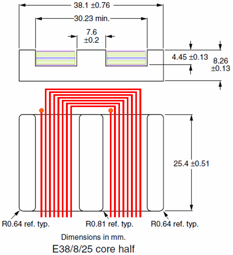
However, it's best to check the data sheet. For a Ferroxcube planar E38/8/25 core-set, you'll see this table below for various different materials including 3F3. Note that the core length (\(\ell_e\)) is 43.7 mm: -

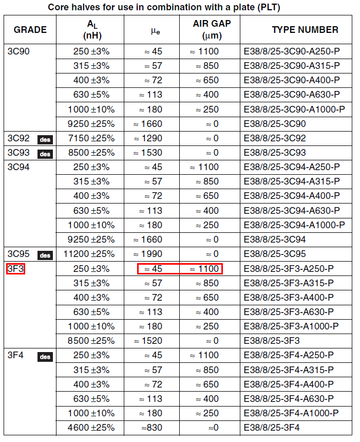
For 3F3 material with a 1.1 mm gap, \(\mu_e\) has fallen to 45 from 1520.

Note that for all the ferrite materials quoted above, the gapped \(\mu_e\) is the same - this is because gapping makes "air" the dominant factor.
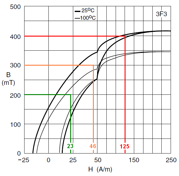
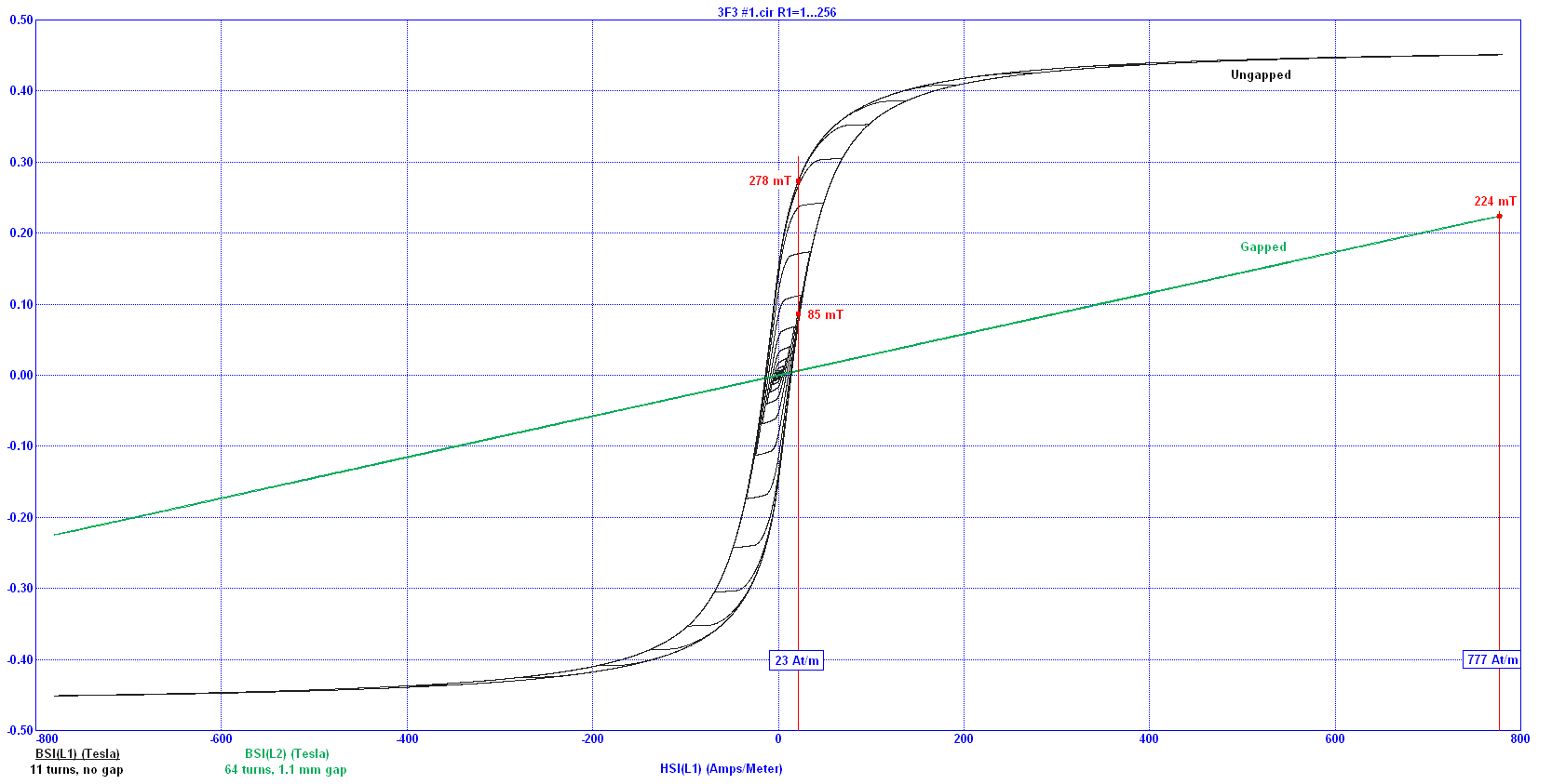
If we now calculate the H-field that produces 200 mT, what was previously 23 At/m is now proportionately higher by 1520 \(\div\) 45 at 777 At/m.

How does this benefit the design of an inductor?

• If the inductor was designed to be 1000 µH (without a gap) we could wind it with 11 turns and get 1029 µH (near enough).

• This is because the \(A_L\) value is 8500 nH for 1 turn and L rises with turns squared hence 11² x 8.5 µH = 1029 µH

• Alternatively we could use the gapped \(A_L\) value of 250 nH. We would now need 64 turns to get an inductance of 1024 µH

For the same 200 mT flux density, comparing 23 At/m (11 turns) and 777 At/m (64 turns) means the gapped inductor realizes a peak current that is about 5.8 times higher than the un-gapped inductor. However, more turns means more copper loss so there is give and take.

____________________________________________________________________________________________________

SIMULATING THE GAPPED AND UNGAPPED 3F3 E38/8/25 CORE-SET

Below is Micro-Cap 12's BH simulation of two inductors placed in series. The black trace is the ungapped 3F3, E28/8/25 core-plate set (11 turns) and the green trace is the 1.1 mm gapped core-plate set (64 turns): -

As can be seen, the previous data sheet calculations are not far off from what a proper detailed simulation produces. For the ungapped core-plate set, due to the large levels of hysteresis, the B-field is somewhere between 85 mT and 278 mT for an applied H-field of 23 At/m. The gapped core-plate set has a much lower hysteresis B-field of about 224 mT for an applied H-field of 777 At/m.

The superb Micro-Cap 12 simulation suite (full version) is now free. See this wikipedia page about Spectrum Software (developers of Micro-cap) for more details. I personally have a debt of gratitude to those involved at Spectrum - it's a great piece of software and you made the world of electronics design a much nicer place to inhabit. For what it's worth, I bought version 9 back in 2008.

____________________________________________________________________________________________________

TEMPERATURE EFFECTS ON MAGNETIC PERMEABILITY

Consider the example of Ferroxcube's 3F3 material and how permeability changes with temperature: -

At 25°C the permeability is 2000 but will rise to about 3300 at 100°C. Clearly this is undesirable when designing an inductor because inductance will rise proportionately. Gapping however comes to the rescue because temperature dependence is reduced by the factor: -

                                                                                         \(\dfrac{\mu_e}{\mu_i}\)

Using the example of the planar 3F3 E38/8/25 core-set discussed previously: -

• The permeability reduced from 1520 to 45 when a 1.1mm gap was introduced

• This is a permeability reduction of 33.8

• The ungapped permeability rose 65% from 2000 to 3300 when temperature changed from 25°C to 100°C

• A gap of 1.1 mm will reduce the 65% change by 33.8 to 1.019%

This is very important to achieving a stable inductor value.

A TRANSFORMER DESIGN 

The Ferroxcube E38/8/25 3F3 core-set is considered: -

• The \(A_L\) figure (1.1 mm air gap) is 250 nH hence, with 64 turns, the inductance is 1024 µH

• With this gap, the maximum H-field is 777 At/m to achieve a \(B_{max}\) of 200 mT (due to \(\mu\) reducing from 1520 to 45)

• With 64 turns and an \(\ell_e\) of 0.0437m, \(I_{max}\) is 777 \(\times\) 0.0437 \(\div\) 64 = 0.531 amps.

The core could surround a primary of 8 PCB layers with 8 turns on each layer. A ninth layer would be required for the secondary winding (assuming that it can be accommodated on one layer). It's tight (and a little hypothetical) but do-able: -