Introduction to Transmission Lines

In 1876 Oliver Heaviside developed the telegrapher's equations. These are still taught today in the theory of transmission lines. Since I learnt them, I've found ways of approaching the subject in a more accessible way. I mean, we study the telegraphers equations usually once in a life time and, when faced with studying them again, it's daunting. So, this page is about showing alternative ways using regular methods familiar to most electrical engineers. What I'm aiming to do is cover four things: -     • Characteristic impedance of a cable     • Reflection coefficient at the load end of the cable     • Velocity of propagation of signals travelling down the cable     • Propagation constant A good place to start is modelling a short section of cable using inductors and capacitors. That model will translate to mathematical expressions. From those we can derive the cable's characteristic impedance. I've chosen to model coaxial cable but equally, twisted-pair would deliver the same result.

Coaxial Cable (inductance)

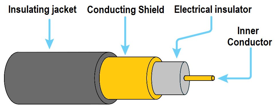
Due to the unique construction of coaxial cable, the entire magnetic field produced is sandwiched between the inner conductor and the outer conducting shield (in the electrical insulator shown above). Note - This assumes that the inner conductor's forward current equals the magnitude of the returning shield current. This isn't an unusual situation of course; this is how we expect (and want) to use coax. So, with equal magnitude (but opposing) currents in the shield and inner conductor, the magnetic field beyond the perimeter of the cable cancels to zero. The impact of this is that the cable inductance "belongs" only to the inner conductor; the magnetic field within does not cause the shield to possess inductance and, it's the same for a current carrying tube; the resulting internal magnetic field is always zero; only an external field is produced. Here's a QuickField example; the image below is of a tube carrying 1000 amps "into the page". The operating frequency is 100 kHz hence, we can determine inductance if we so desired. I used the student edition of Quickfield and, not unexpectedly, it's a tad limited in the number of nodes it can calculate: -

Note 1 - Quickfield is a 2-dimensional (x and y) field plotter that assumes an infinite z-axis (in and out of the page). Calculated values (such as voltage) are based on a 1 metre length in the z-axis. So, for instance, voltages shown in the images are "per metre". These were measured using QuickField's "local values" facility (point and click). Note 2 - The flux density colour range is deliberately limited hence, anything above 10 mT is shown red. This is a deliberate action so that the corner regions (where flux density drops below 10 mT) can be easily compared to those in the next image. The key point is that flux density magnitude (external to the cable) is identical for both images. Note 3 - The other key point is that there is no magnetic field within the tube (above) and, because coaxial cable (when used correctly) generates no external magnetic field, the shield inductance has to be zero More on this further down.. Here's the field-plot when the inner conductor is carrying 1000 amps and the shield is "open circuit": -

Note 1 - the voltage required to deliver 1000 amps through the inner is 274.9 volts per metre. Yet, for the shield, the equivalent drive level is only 95.9 volts per metre. This should immediately tell you that the inductance of the shield is much lower than the inductance of the inner. This fact is also fundamental in understanding skin effect in solid conductors. In other words, for a given AC drive voltage, current will preferentially flow in the outer regions of a conductor. Note 2 - if you compare flux density colours in the corners you can see that the two scenarios produce the same flux density external to the cable at any point in space. Key points regarding the images above: -     • An internal magnetic field is only produced by the inner conductor (as one would expect)     • The external magnetic field magnitudes from inner and shield are identical     • Consistent flux density colour ranges are used (0 mT to 10 mT)     • Because shield and inner currents are opposing, the external magnetic field cancels to zero And, just in case you weren't convinced about the cancellation, here's a field-plot with +1000 amps on the inner and -1000 amps on the shield. Clearly, there is only a magnetic field between inner and shield: -

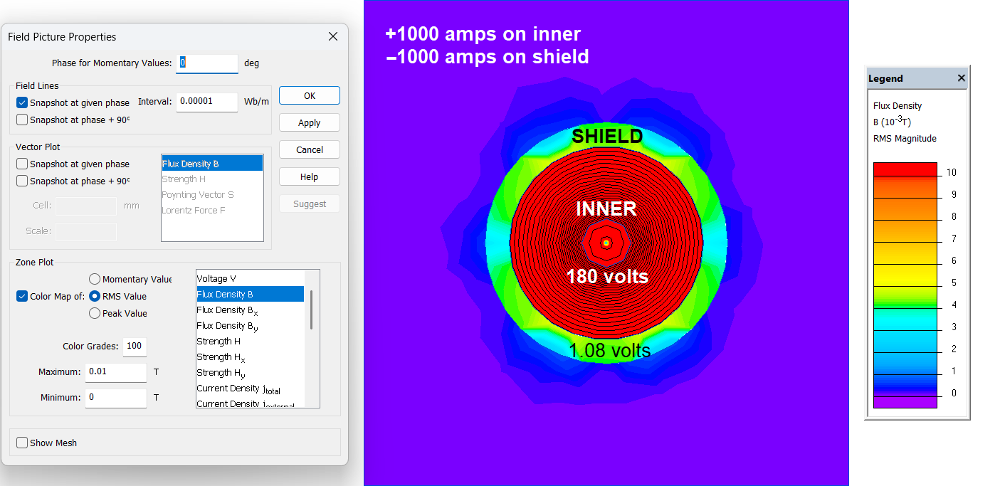
Note 1 - For the final image above, the voltage value on the inner conductor was 180 volts per metre and, given that the analysis frequency was set to 100 kHz (with 1000 amps flowing), the inductance comes out at 286 nH per metre. The QuickField model does not accurately represent any particular coaxial cable so, that figure is just useful to know. Note 2 - The shield is at 1.08 volts so, compared to the inner, the reactance is massively less. More than likely it's just the resistance of a 1 metre copper tube mixed with some small errors using the limited capabilities of QuickField's student edition. So, we have the very desirable situation of the shield being regarded as "0 volts" along its whole length. For a non-ideal coaxial cable, the shield's series resistance will drop a small voltage but, we generally consider coaxial cable to have inductance associated only with the inner conductor.

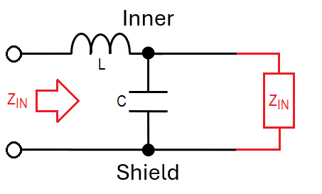
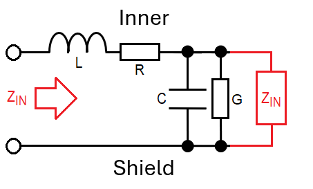
Coaxial Cable (lossless lumped-element model)

For cable capacitance, it's fairly easy to see that it exists between inner and shield so now, we can make an equivalent electrical circuit for a length of cable. It can be regarded as a distributed network of inductors and capacitors (called a lumped-element model): -

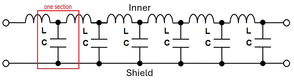
Note - The lumped element model was first proposed by Lord Kelvin in 1854 and, later developed by Heaviside. Each section (shown above in the red box above) is symmetrical hence, its input impedance (on the left) is identical to its output impedance. We can therefore analyse one section feeding a load of \(Z_{IN}\) where \(Z_{IN}\) represents the input impedance of the next section: -

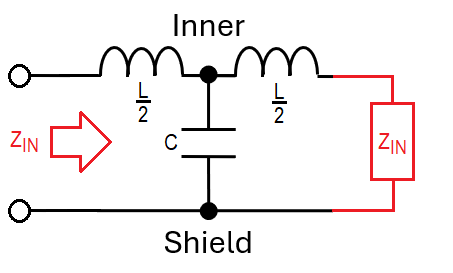
Using parallel and series circuit knowledge, we can evaluate \(Z_{IN}\): - $$Z_{IN} = \dfrac{j\omega L}{2} + \dfrac{\frac{1}{j\omega C}\cdot\left(\frac{j\omega L}{2}+Z_{IN}\right)}{\frac{1}{j\omega C}+\frac{j\omega L}{2}+Z_{IN}}$$ $$Z_{IN}\dfrac{1}{j\omega C} +Z_{IN}\dfrac{j\omega L}{2}+Z_{IN}^2 =Z_{IN}\dfrac{j\omega L}{2}+\dfrac{j^2\omega^2L^2}{4}+\dfrac{L}{2C}+\dfrac{L}{2C}+Z_{IN}\frac{1}{j\omega C}$$ $$Z_{IN}^2 = \dfrac{j^2\omega^2L^2}{4}+\dfrac{L}{C}$$ We now consider L and C diminishing to zero i.e. the cable is no longer built from lumped L and C impedances but, represented homogeneously. When this happens the \(\frac{j^2\omega^2L^2}{4}\) term becomes vanishingly small compared to \(\frac{L}{C}\) and we end up with this: - $$\boxed{Z_{IN} = \sqrt{\frac{L}{C}}\hspace{1cm}\color{red}{\text{we call this the characteristic impedance of the cable }}(Z_0)}$$ However, this formula only applies to a line that doesn't have copper and dielectric losses. Nevertheless, it's an important, valid and useful equation for most situations above 100 kHz. Because cable suppliers state the capacitance and inductance per metre, we can use those values in the formula. So, for a 50 Ω coaxial cable, C will typically be 100 pF/m and, L will typically be 250 nH/m: - $$Z_{0} = \sqrt{\frac{250\times 10^{-9}}{100\times 10^{-12}}} = 50 \text{ }\Omega$$ What does this mean; if we had an infinite length of 50 Ω coaxial cable and applied 1 volt we would see 20 mA flow indefinitely. Clearly, we don't have an infinite length of cable but we can draw conclusions. For a short length of cable, 20 mA would flow upon applying 1 volt for several nanoseconds. It's important to recognize that the load cannot intially influence the current flow. So, after a few nano seconds delay, 1 volt and 20 mA reach the load at the end of the cable. The problem that then arises is how we deal with those signals when the load impedance (\(Z_L\)) isn't 50 Ω because, it appears to be violating Ohm's Law.

Reflection coefficient (avoiding the violation of Ohm's Law)

Previously, it was discussed that the initial current that flows is independant of the load impedance (\(Z_L\)) and, this could produce an anomaly if \(Z_L\) was not identical to the cable's characteristic impedance (\(Z_0\)). To solve this we can set up a thought experiment: -     •  Assume a cable of characteristic impedance \(Z_0\)     •  Assume an applied voltage (\(V_F\)) at one end of the line     •  The current (\(I_F\)) that initially flows equals \(V_F\) divided by \(Z_0\) When the voltage and accompanying current reach the end of the cable and meet \(Z_L\) there may be a violation of Ohm's law if \(Z_0\) does not equal \(Z_L\). This is the potential violation that we have to fix. For instance, if \(Z_L\) > \(Z_0\) we have to consider a mechanism that prevents that violation: -     •  Adjust the voltage arriving at \(Z_L\) to be bigger and, at the same time     •  Adjust the current arriving at \(Z_L\) to be smaller     •  Adjust voltage and current in such a way so that we achieve a ratio of \(Z_L\)     •  Those adjustments are somehow "dealt with" Using \(\delta\) to "fudge" the numbers, algebraically we could make the adjustments like this: - $$\dfrac{V_F + \delta V_F}{I_F - \delta I_F} = Z_L = \text{fixing the Ohm's law violation}$$ \(\delta\) increases the load voltage and decreaes the load current (the fudge) to match ZL (the load) $$\therefore \dfrac{V_F}{I_F}\cdot \dfrac{1 + \delta}{1 - \delta} = Z_L\hspace{1cm}\longrightarrow\hspace{1cm} Z_0\cdot \dfrac{1 + \delta}{1 - \delta} = Z_L$$ $$\text{Hence,}\hspace{1cm}\delta Z_0 +\delta Z_L\hspace{1cm} =\hspace{1cm} Z_L - Z_0$$ $$\boxed{\text{And,}\hspace{1cm}\delta = \dfrac{Z_L-Z_0}{Z_L+Z_0}\hspace{1cm}\color{red}{\text{we call this the reflection coefficient }}(\Gamma)}$$ Note - The \(\delta\) symbol is just an invented device to get through the thought experiment. The important subtlety that prevents an Ohm's law violation is the "bit" we add to voltage and, the "bit" we subtract from current i.e. \(\delta V_F\) and \(\delta I_F\). Clearly their ratio is \(Z_0\) and, this means that they can naturally flow (together) back into the cable because they have the correct ratio to do so. That is called a reflection and, it travels from the load back to source. Indeed, if the source isn't matched to \(Z_0\), reflections can rattle back and forth for some time and, cause significant signal disruptions. They eventually die down due to propagation losses. When \(Z_0 > Z_L\) then, \(\Gamma\) will be negative. When \(Z_0 = Z_L\) then, \(\Gamma\) will be zero.

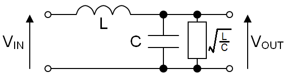
Coaxial Cable (modified model)

This is the circuit model I used earlier to derive the characteristic impedance \(Z_0 \): -

Below is an alternative. I'm introducing this alternative because it more readily lends itself to analysing the velocity of propagation (shown in a later section): -

$$Z_{IN} = j\omega L + \dfrac{\frac{1}{j\omega C}\cdot\left(Z_{IN}\right)}{\frac{1}{j\omega C}+Z_{IN}}$$ $$\frac{Z_{IN}}{j\omega C} +Z_{IN}^2 =Z_{IN}\cdot j\omega L+\frac{L}{C}+\frac{Z_{IN}}{j\omega C}$$ $$Z_{IN}^2 = Z_{IN}\cdot j\omega L+\dfrac{L}{C}$$ As before we consider L and C diminishing to zero i.e. the cable is no longer built from lumped L and C impedances but, represented homogeneously. When this happens the \(Z_{IN}\cdot j\omega L\) term becomes vanishingly small compared to \(\frac{L}{C}\) and we end up with this: - $$\boxed{Z_{IN} = \sqrt{\frac{L}{C}}\hspace{1cm}\text{i.e. the same as before }}$$ In effect, it doesn't matter which model you use because both have the same value of \(Z_0\).

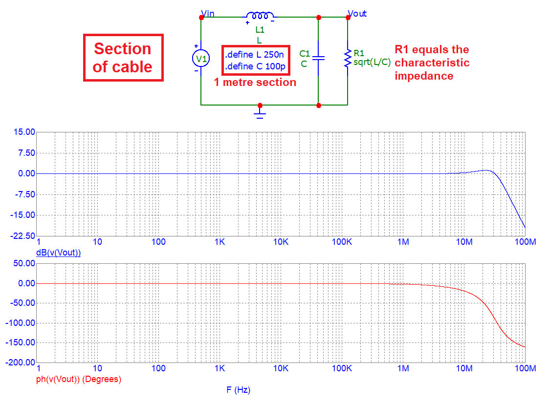
Velocity of propagation (simulator result)

How quickly do the voltage and current signals travel down a coaxial cable? So far we have found the characteristic impedance (\(Z_0\)) and the reflection coefficient (\(\Gamma\)) and, through experience, we know that electricity travels quickly but, how quickly? My preferred method for finding \(VoP\) is: -     •  Derive the transfer function for a 1 metre section of cable (see below image)     •  This yields a formula for the output phase lag and,     •  With a little more manipulation, the time delay for the 1 metre cable is found     •  The inverse of time lag for 1 metre of cable is the velocity of propagation To help, we can use a simulator to get a feel for the phase lag. I've picked values typical of a 50 Ω cable and, I'm using a simulator because it's easy show how phase shift manifests. Importantly, I'm using the alternative model of a transmission line segment (that was mentioned earlier): -

The bode-plot above doesn't seem to yield much useful information until we focus much more closely on the phase response plotted linearly against frequency up to 1 MHz (an arbitrary limit). We need to look at the phase change minutiae to reveal what we wish to see: -

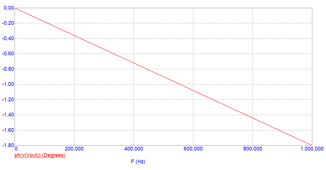
•  At 1 MHz, the phase lag of the output is 1.8° (compared to the input)     •  As a fraction of the period (1 µs) it's 0.005 hence, it's a time lag of 5 ns (1 µs \(\times\frac{1.8}{360}\))     •  At 100 kHz, the phase lag is 0.18° but, it's still a time lag of 5 ns (10 µs \(\times\frac{0.18}{360}\))     •  The time lag equals 5 ns all the way to 1 MHz (an arbitrary limit)     •  If we went much higher than 1 MHz, the phase response becomes non-linear With a 5 ns time lag and a 1 metre section of capacitance and inductance, the velocity of propagation is 200 million metres per second. This is two-thirds of the speed of light for comparison. If we'd modelled (say) 10 cm of cable, the new time lag (0.5 ns) would remain constant all the way to over 10 MHz. However, when considering 1 metre of cable modelled from ten 10 cm sections, the time lag would still equal 5 ns. So, it's arbitrary how much cable you model. The point of simulation is that it demonstrates the linearity of phase lag at "lower frequencies". The math that follows does the same; the phase lag formula becomes intentionally restricted to "lower frequencies". This may seem problematic but, if we modelled a 1 mm section of cable we would get a time lag of 5 ps and, when we bolted together 1000 such sections we would be back to a time lag of 5 ns. A 1 mm section would have a natural resonant frequency of tens of GHz and, the term "lower frequencies" would be from DC to 1 GHz (linear phase against frequency). But why stop there; we could model sections of 0.01 mm and we would find that an acceptable "lower frequency limit" is 100 GHz. It's just an arbitrary point and has zero effect when we assume the cable moves from lumped LC values to a homogeneous distribution of L and C. What follows is a more mathematical approach that relies on knowledge of 2nd order filters...

Velocity of propagation (mathematical proof)

A simulator is great for demos but, a phase angle formula is needed to understand the true dependencies. The modelled section (used above) can be analyzed as a simple 2nd order low pass filter and, if you went through the derivation (omitted for brevity) you will find this: -

$$\text{Phase lag} = \arctan\left(\dfrac{2\zeta\dfrac{\omega}{\omega_n}}{1 - \dfrac{\omega^2}{\omega_n^2}}\right)$$ We can simplify this equation because we are considering the situation where \(\omega\) is a lot smaller than \(\omega_n\): -     •  Arctan(small number) is the small number because the powers of \(x\) are insignificant: - $$\arctan(x) = x - \frac{x^3}{3} + \frac{x^5}{5} - ...$$     •  The denominator equals 1 (because \(\omega\) is so much smaller than \(\omega_n\)) hence: - $$\text{Phase lag} = {2\zeta\dfrac{\omega}{\omega_n}}$$ From filter theory we know that the damping factor (\(\zeta\)) for a parallel tuned circuit is this: - $$\zeta = \dfrac{1}{2\cdot R}\sqrt{\dfrac{L}{C}}$$ And, of course, \(R=Z_0\) hence: - $$\zeta\hspace{1cm} = \hspace{1cm}\dfrac{1}{2\cdot\sqrt{\dfrac{L}{C}}}\sqrt{\dfrac{L}{C}}\hspace{1cm} = \hspace{1cm}0.5$$ This implies: - $$\text{Phase lag} = {\dfrac{\omega}{\omega_n}}$$ From filter theory, we know that \(\omega_n\) equals \(\dfrac{1}{\sqrt{LC}}\) hence: - $$\boxed{\text{Phase lag} = \omega\sqrt{LC}}$$ Anyone studying transmission lines will recognize this as the imaginary part of the propagation constant (\(\gamma\)). Its proper name is the phase constant, \(\beta\). The real part of \(\gamma\) being called the attenuation coefficient, \(\alpha\). For a lossless line, \(\alpha\) is unity. Dividing the phase lag by \(\omega\) gives us the time lag: - $$\text{Time lag} = \sqrt{LC}$$ And, the velocity of propagation is the reciprocal of the time lag (for a 1 metre length of cable): - $$\boxed{\color{red}{\text{Velocity of propagation}} = \dfrac{1}{\sqrt{LC}}}$$ Note - Because we are talking about velocity, L and C are the equivalent 1 metre values. If we used the previous values for L and C (250 nH/m and 100 pF/m) we also get a velocity of propagation of 200 million metres per second (two-thirds the speed of light). So far we have derived the loss-less charactristic impedance (\(Z_0\)), the reflection coefficient (\(\Gamma\)) and, the loss-less velocity of propagation (\(V_P\)) using hopefully a fairly minimalistic approach to the math. I've focused on coaxial cable for the above explanations but, twisted pair (shielded or otherwise) can be analysed in exactly the same way and, the formulas derived are the same.

Lossy line characteristic impedance

The lossy model has two new components labelled R and G (where G is a resistor of value 1/G): -

$$Z_{IN}\hspace{5mm} =\hspace{5mm} R+j\omega L +Z_{IN}||\dfrac{1}{G+j\omega C}\hspace{5mm} = \hspace{5mm}R+j\omega L +\dfrac{\frac{Z_{IN}}{G +j\omega C}}{Z_{IN}+\frac{1}{G +j\omega C}}$$ $$Z_{IN}\hspace{5mm} =\hspace{5mm} R+j\omega L\hspace{5mm} +\hspace{5mm}\dfrac{Z_{IN}}{1+Z_{IN}(G +j\omega C)}$$ $$Z_{IN}+Z_{IN}^2(G +j\omega C)\hspace{5mm} =\hspace{5mm} (R+j\omega L)\cdot\left[1+Z_{IN}(G +j\omega C)\right]+Z_{IN}$$ $$Z_{IN}^2(G +j\omega C)\hspace{5mm} =\hspace{5mm} R+j\omega L + Z_{IN}\left[(R+j\omega L)(G +j\omega C)\right]$$ $$Z_{IN}^2\hspace{5mm} =\hspace{5mm} \dfrac{R+j\omega L}{G +j\omega C} + Z_{IN}(R+j\omega L)$$ As before, when we diminish the 4 component parts of the line section towards zero, \(Z_{IN}(R+j\omega L)\) becomes vanishingly small and, we end up with an equation we should all be familiar with: - $$\boxed{\hspace{5mm}Z_{IN}\hspace{5mm} =\hspace{5mm} \sqrt{\dfrac{R+j\omega L}{G +j\omega C}}\hspace{5mm} =\hspace{5mm}Z_0\hspace{5mm}}$$

Lossy line propagation constant

The propagation constant (\(\gamma\)) shapes how a signal evolves as it passes down a transmission line. It is used (along with distance) in an exponential formula shown further down. But, before we get to that, we should examine a short line formed from R, L, G and C and derive a formula for \(\gamma\): -

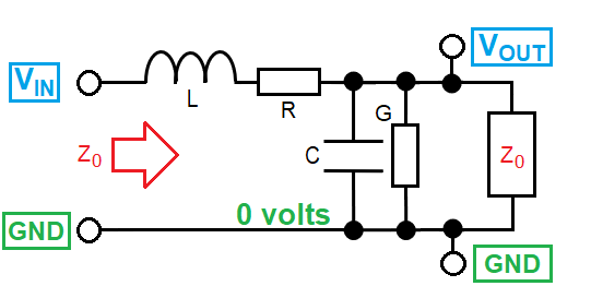
Note 1 - Output impedance \(Z_0\) represents the loading from the cable that follows. Note 2 - the values of R, L, G and C shown above are for a very short/miniscule line. So, you could begin with the voltage transfer function (a potential divider) like this: - $$\dfrac{V_{OUT}}{V_{IN}}\hspace{0.5cm}=\hspace{0.5cm} \dfrac{Z_0||\frac{1}{G+j\omega C}}{R+j\omega L + Z_0||\frac{1}{G+j\omega C}} \hspace{0.5cm}=\hspace{0.5cm}\frac{\text{parallel parts (G, C & }Z_0\text{)}}{\text{series parts (R & L) + parallel parts}}$$ But, it can be looked at in a simpler way. For instance, when R, L, G and C are very small, we know that the denominator (series parts + parallel parts) is \(Z_0\) hence: - $$\dfrac{V_{OUT}}{V_{IN}}\hspace{1cm}=\hspace{1cm} \dfrac{Z_0||\frac{1}{G+j\omega C}}{Z_0}$$ Likewise, the numerator can also be simplified to \(Z_0-(R+j\omega L)\): - $$\dfrac{V_{OUT}}{V_{IN}}\hspace{1cm}=\hspace{1cm} \dfrac{Z_0 - (R+j\omega L)}{Z_0}\hspace{1cm} =\hspace{1cm} 1 - \dfrac{R+j\omega L}{Z_0}$$ We can now introduce \(Z_0\) that was derived in the previous section: - $$\dfrac{V_{OUT}}{V_{IN}}\hspace{1cm}=\hspace{1cm} 1 - (R+j\omega L)\cdot\sqrt{\dfrac{G+j\omega C}{R +j\omega L}}$$ As stated earlier, we are intentionally analysing a very short section of transmission line but, there is a potential problem in merging the very short "\(R+j\omega L\)" with the "1 metre" values normally implied by \(Z_0\). We can resolve this with a new term (\(\delta\)). The new term links with the "\(R+j\omega L\)" that is external to the similar terms within \(Z_0\). In effect, the external "\(R+j\omega L\)" values can be "per metre" providing they are "shortened" by \(\delta\). In effect, \(\delta\) is used to make the analysed line section miniscule. We now have this: - $$\dfrac{V_{OUT}}{V_{IN}}\hspace{0.9cm}=\hspace{0.9cm} 1 - \delta\sqrt{(R+j\omega L)\cdot(G+j\omega C)}$$ At this point we introduce the expontial equation (containing \(\gamma\) and distance) mentioned above: - $$V_{OUT}(x)\hspace{1cm}=\hspace{1cm} V_{IN}\cdot e^{-\gamma x}$$ The above formula defines \(V_{OUT}\) at distance \(x\) from \(V_{IN}\) and rearranges to: - $$log_e\left(\dfrac{V_{OUT}}{V_{IN}}\right)\hspace{1cm}=\hspace{1cm} -\gamma x$$ We can replace \(\frac{V_{OUT}}{V_{IN}}\) with the R, L, G & C value developed above: - $$log_e\left(1 - \delta\sqrt{(R+j\omega L)\cdot(G+j\omega C)}\right) \hspace{1cm}=\hspace{1cm} -\gamma x$$ Because the 1 metre values of R, L, G and C are reduced to miniscule values by the introduction of \(\delta\), the \(log_e\) side of the equation simplifies to this: - $$-\delta\sqrt{(R+j\omega L)\cdot(G+j\omega C)}\hspace{1cm}=\hspace{1cm} -\gamma x$$ Note - This is because \(log_e(1-y)\) expands to \(-y-\frac{y^2}{2}-\frac{y^3}{3}-...\) and, in particular, when \(y\) is miniscule, we can ignore the terms containing powers of \(y\). Recognizing that \(x\) and \(\delta\) both describe the same miniscule length of line, it follows that: - $$\boxed{\hspace{0.5cm}\gamma \hspace{1cm}=\hspace{1cm} \sqrt{(R+j\omega L)\cdot(G+j\omega C)}\hspace{0.5cm}}$$ As implied above, the use or meaning of \(\gamma\) outside of an exponential equation is somewhat limited. The R, L, G and C values contained in \(\gamma\) are "per metre" values but, without distance (\(x\) or \(\delta\)), there is no clear meaning. So, the correct and proper use of the propagation constant is this: - $$\boxed{\hspace{5mm}V_{OUT}(x) \hspace{1cm}=\hspace{1cm} V_{IN}\cdot e^{-x\sqrt{(R+j\omega L)\cdot(G+j\omega C)}}\hspace{5mm}}$$ A couple of examples follow that show how things pan-out in different scenarios.

Demonstrating \(\gamma\) on a loss-only line

Let's start simple with a hypothetical t-line model made purely from resistive components (R & G) hence, there is no phase shift (zero time lag end-to-end). I'm demonstrating the precision of the \(\gamma\) formula against a micro-cap simulation where \(\gamma = \sqrt{RG}\): -

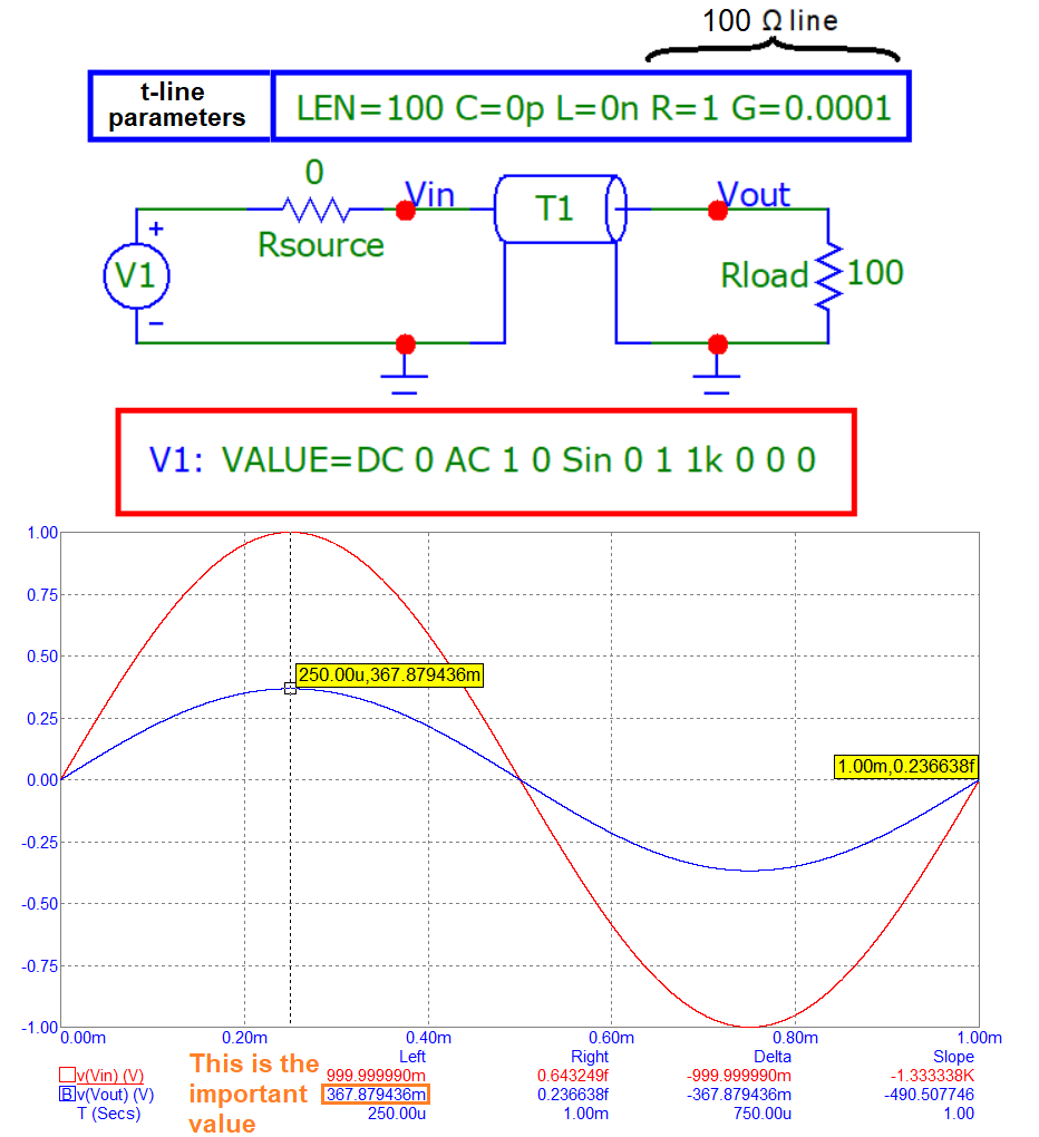
The t-line is 100 metres long (LEN) and has only resistive values (R = 1 and G = 0.0001). Those values produce a characteristic impedance of 100 Ω hence, the t-line is terminated by that value. Source \(V_{IN}\) is a 1 kHz sinewave of 1 volt peak amplitude and, \(V_{OUT}\) is 367.879436 mV peak. Both input and output waveforms are totally in-phase because, C and L are set to zero. Now, if we use the exponential formula that incorporates \(\gamma\) we get this: - $$V_{OUT}\hspace{0.5cm}=\hspace{0.5cm} V_{IN}\cdot e^{-x\sqrt{RG}} \hspace{0.5cm}=\hspace{0.5cm}\text{ 1 volt}\cdot e^{-100 \sqrt{0.0001}} \hspace{0.5cm}=\hspace{0.5cm}0.36787944 \text{ volts}$$ That's "case proven" for the purely resistive line but, it's more complicated when R, L, G and C are all present. This is because \(\gamma\) is a complex number defining both (\(\alpha\)) and phase shift (\(\beta\)): - $$V_{OUT}(x) \hspace{1cm}=\hspace{1cm} V_{IN}\cdot e^{-x\gamma}\hspace{0.5cm}\rightarrow\hspace{0.5cm}V_{IN}\cdot e^{-x(\alpha +j\beta)}$$ More on \(\alpha\) and \(\beta\) in the next section but, note that the value of \(\gamma\) used above (\(\sqrt{RG}\)) is purely \(\alpha\).

Demonstrating \(\gamma\) on a loss-less line

The t-line is made exclusively from reactive components (L and C) hence, there is no attenuation (\(\alpha\)). The micro-cap simulation uses a 1 MHz source frequency that has a peak amplitude of 1 volt. The length of the line (LEN) is 10 metres. L and C are chosen for a 50 Ω characteristic impedance: -

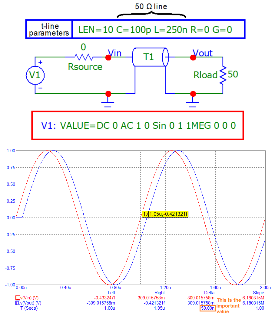
It should be clear that \(V_{OUT}\) is unattenuated but, has a noticeable phase shift. If you now look at the "delta" column beneath the waveform plot you will see a highlighted number. That number is 50 ns and is the time lag of \(V_{OUT}\) compared to \(V_{IN}\). What does this tell us? Going back to the derivation of \(\gamma\) we have this: - $$\gamma \hspace{1cm}=\hspace{1cm} \sqrt{(R+j\omega L)\cdot(G+j\omega C)}$$ Then, if R and G were made zero we get this: - $$\gamma \hspace{1cm}=\hspace{1cm} \sqrt{(j\omega L)\cdot(j\omega C)} \hspace{1cm}=\hspace{1cm} j\omega\sqrt{LC}\hspace{1cm}=\hspace{1cm} j\beta$$ We know the values of \(\omega\), L and C so, plugging in the numbers we get: - $$j(2\pi\times 10^6\sqrt{250\times 10^{-9}\times 100 \times 10^{-12}}) \hspace{0.25cm}=\hspace{0.25cm} j(6.283185\times 10^6 \times 5\times 10^{-9}) \hspace{0.25cm}=\hspace{0.25cm} j\dfrac{\pi}{100}$$ This is a phase shift of \(\frac{\pi}{100}\) radians or 1.8°. It's a phase shift because of how it is used within the exponential formula. In other words, if we multiply a signal by \(e^{-j\theta}\), we rotate that signal through a phase angle of \(\theta\). We don't need to calculate \(e^{-j\theta}\); just recognize that the important part is phase shift \(\theta\). Note - 1.8° is the same value in the "velocity of propagation" section (derived using L = 250 nH, C = 100 pF and f = 1 MHz). Returning to the simulation result, because the t-line is 10 metres long we get an overall phase shift that is ten times greater at 18°. At 1 MHz, that's a time delay of 50 ns (as per the simulation). April 25th 2026

A deeper dive into \(Z_0,\gamma, \alpha \text{ and }\beta\)

Section added April 29th 2026 Many articles on the subject state that \(\gamma=\sqrt{(R+j\omega L)(G+j\omega C)}\) but, a simpler form is informative when studying \(\alpha\) and \(\beta\). If you scroll back to an earlier section I derived this: - $$\dfrac{V_{OUT}}{V_{IN}}\hspace{1cm} =\hspace{1cm} 1 - \dfrac{R+j\omega L}{Z_0}$$ But, instead of substituting the derived version of \(Z_0\), we could develop the propagation constant to be: - $$\gamma \hspace{1cm} =\hspace{1cm} \dfrac{R+j\omega L}{Z_0}$$ Note - R and L terms are the full "per metre" values (in case there is any doubt). Then, recognizing that for most scenarios \(Z_0\) is fully resistive, we are able to say this: - $$\alpha = \frac{R}{Z_0}\hspace{1cm}\text{and}\hspace{1cm}\beta = \frac{\omega L}{Z_0}$$ However, there are two cases when \(Z_0\) becomes a complex value: -     •   Above 1 GHz when cable dielectric losses associated with \(G\) are rising and,     •   At audio frequencies when the magnitude of \(\omega L\) drops towards the value of \(R\) Note - it may seem trivial to consider audio frequencies but, in the case of telephony (and the reduction of earpiece sidetone), recognizing the complex nature of the cable's characteristic impedance is important. A revealing exercise is to convert \(Z_0\) into its polar co-ordinates: - \(\sqrt{\dfrac{R+j\omega L}{G+j\omega C}} \hspace{1mm}\rightarrow\hspace{1mm} \sqrt{\dfrac{(R+j\omega L)(G-j\omega C)}{G^2+\omega^2 C^2}} \hspace{1mm}\rightarrow\hspace{1mm} \sqrt{\dfrac{RG+\omega^2 LC+j\omega(LG-CR)}{G^2+\omega^2 C^2}}\tag{Zo}\) So now we can extract the phase angle: - $$\angle = \sqrt{Tan^{-1}\left(\dfrac{\omega(LG-CR)}{RG+\omega^2LC}\right)}$$ If you understand phasors, the square root of an angle is half the angle hence: - $$\boxed{\hspace{5mm}\angle \hspace{5mm}=\hspace{5mm} \dfrac{Tan^{-1}\left(\dfrac{\omega(LG-CR)}{RG+\omega^2LC}\right)}{2}\hspace{5mm}}$$ Note - if \(LG=CR\) then there is zero phase shift. This is called a "distortionless line". Consequently, all signal frequencies travel at the same speed hence, there is no signal dispersion. Oliver Heaviside developed a solution that used this condition to improve signal integrity on long telegraph lines. At appropriate distances inductors were added to the cable. To find \(Z_0\)'s magnitude, take the square root of the squared numerator terms in equation (\(Zo\)): - $$|Z_0| =\sqrt{\dfrac{\sqrt{R^2G^2+2\omega^2 LCRG + \omega^4L^2C^2 + \omega^2(L^2G^2+C^2R^2-2LGCR)}}{G^2+\omega^2C^2}}$$ $$|Z_0| =\sqrt{\sqrt{\dfrac{R^2G^2 + \omega^4L^2C^2 + \omega^2(L^2G^2+C^2R^2)}{(G^2+\omega^2C^2)(G^2+\omega^2C^2)}}}$$ The "trick" is recognizing that \((G^2+\omega^2C^2) \times (R^2+\omega^2L^2)\) equal the numerator hence: - $$\boxed{\hspace{5mm}|Z_0| \hspace{5mm}=\hspace{5mm} \sqrt{\sqrt{\dfrac{R^2+\omega^2L^2}{G^2+\omega^2C^2}}}\hspace{5mm}}$$ Spreadsheet graph demonstrating impedance magnitude and phase angle at low frequencies: -

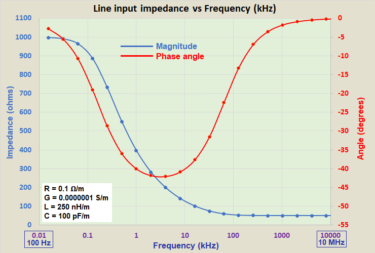
Points to interest: -     •   By 10 MHz the cable has a characteristic impedance that is reliably resistive     •   I wouldn't worry too much if 1 MHz was also regarded as being purely resistive     •   The maximum phase change (42°) occurs around 3 kHz     •   At 3 kHz, phase change is governed by R and C with \(\angle\) tending to \(\sqrt{-j}\) or -45°     •   \(Z_0\) above 10 MHz is 50 Ω (as we would expect)     •   \(Z_0\) tends towards 1000 Ω at low frequencies (as we would expect)

Reflection coefficient and signal power

Section added April 29th 2026 The flow of a signal down a cable is a transmision of power. The amount of power initially transmitted is volts squared (\(V_F^2\)) divided by \(Z_0\). Likewise, the power received by the load is \(V_L^2/Z_L\) and, the reflected power is \(V_R^2/Z_0\). We can equate these powers: - $$\dfrac{V_F^2}{Z_0}-\dfrac{V_R^2}{Z_0} = \dfrac{V_L^2}{Z_L}$$     •   \(V_F\) is the forward (load bound) voltage     •   \(V_R\) is the reflected (source bound) voltage when there is a mismatch     •   \(V_L\) is the load voltage (the sum of \(V_F\) and \(V_R\)) From this we can define \(V_R=V_L-V_F\) hence: - $$\dfrac{V_F^2}{Z_0}-\dfrac{(V_L-V_F)^2}{Z_0}  =  \dfrac{V_L^2}{Z_L}$$ $$\dfrac{V_F^2}{Z_0}-\dfrac{V_L^2-2V_FV_L+V_F^2}{Z_0}  =  \dfrac{V_L^2}{Z_L}$$ $$-\dfrac{V_L^2}{Z_0}+\dfrac{2V_FV_L}{Z_0}  =  \dfrac{V_L^2}{Z_L}$$ $$\dfrac{2V_FV_L}{Z_0}  =  \dfrac{V_L^2}{Z_L} + \dfrac{V_L^2}{Z_0}$$ $$\dfrac{2V_F}{Z_0}  =  \dfrac{V_L}{Z_L} + \dfrac{V_L}{Z_0}$$ $$2V_F  =  V_LZ_0\left(\dfrac{1}{Z_L}+\dfrac{1}{Z_0}\right) = V_L\left(\dfrac{Z_L+Z_0}{Z_L}\right)$$ $$\boxed{ \text{Hence} V_L  =  V_F\dfrac{2Z_L}{Z_L+Z_0}  =  V_F(1+\Gamma) }$$ One observation is that if \(Z_L\) is open-circuit, \(\Gamma\) equals +1 and, \(V_L\) is double \(V_F\). This is convenient when transmitting data because, we can use a series terminator equal to \(Z_0\) at the sending end and, receive an uncorrupted logic level signal at the receiving end. There is a reflection that travels back to the source but, the series source terminator will prevent subsequent reflections "bouncing" back to the load. So, if the logic level is 5 volts and we use a series terminator matching \(Z_0\), the logic level transmitted is only 2.5 volts but, this doubles to 5 volts at the load/receiver when \(Z_L\) is open-circuit. Recalling that we defined \(V_R=V_L-V_F\) then we can also determine \(V_R\): - $$\boxed{ V_R=V_F(1+\Gamma)-V_F = V_F\cdot\Gamma }$$ Note - For lossy lines, the value we use for \(V_F\) is just before it hits the load i.e. the attenuated value.

What's left to say?

There's plenty left to cover and, as time passes I'm sure I'll add to this. What springs to mind are these uncovered areas: -     •   Input impedance when driven by a sinewave     •   Quarter wave transformners     •   Standing waves More to come...